National Weather Service Training Center

Basic Hydrologic Concepts

Section III

Important Aspects of the Hydrologic Cycle

The Hydrologic Cycle

And

Determination of Mean Areal Precipitation

Introduction

The hydrologic cycle is the process where water is circulated through the earth-ocean-atmosphere system from the oceans to the air and then to the land in the form of rain or snow. Understanding the various components of the hydrologic cycle is important to forecasters who must supply hydrologic forecasts and information to external users.

The process of changing precipitation to runoff is one of the most important components of the hydrologic cycle. Hydrologic models attempt to simulate various components of the hydrologic cycle including the runoff process. Lumped parameter models utilize values averaged over a given area. There are various methods for determining average values of a parameter such as rainfall over a catchment area.

Objectives

At the conclusion of this module, you should be able to:

· Define the hydrologic cycle.

· Describe the major components of the hydrologic cycle affecting the flow of rivers and streams.

· Define MAP (Mean Areal Precipitation).

· Describe methods the RFC uses to compute MAP.

· Describe the method to compute MAP from the NEXRAD precipitation estimates.

Components of the Hydrologic Cycle

The hydrologic cycle is the process where water is circulated through the earth-ocean-atmosphere system from the oceans to the air and then to the land in the form of rain or snow. This is a closed system where the amount of water is constant.

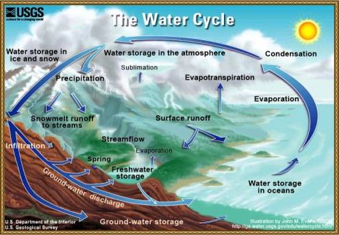
Source: USGS

Baseflow is where the water table intersects a stream channel-groundwater and enters the stream via springs.

Drainage Basin is an area on the earth’s surface over which water flows toward a common outlet or exit point.

Evaporation moves water from the ocean and land surface to the atmosphere.

Evapotranspiration plays a small part, largely due to its impact on soil moisture content affecting infiltration rates, and is a complex process affected by factors such as:

· Availability of heat energy from the environment

· Humidity

· Wind

· Soil type

· Time of year

· Amount and type of vegetation

· Amount of available water

Lowest in the winter, peaks in the summer

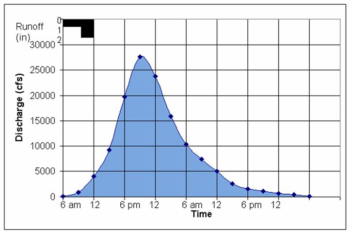
Flood Hydrology is related to interflow and surface runoff. These factors are direct response to a rainfall or snowmelt event.

Gravity is a force or movement of water in a downward direction.

Groundwater Flow moves water through the subsurface to river channels when water cannot percolate downward, collects, and forms groundwater.

Infiltration moves water from the land surface into the soil; governed by soil type and soil moisture.

Interflow is water that enters the soil, percolates a short distance, and then moves horizontally to the stream channel due to a much less pervious soil (pervious: capable of transmitting water).

· Directly contributes to the amount of water found in a river

· Direct response to rainfall and snow melt

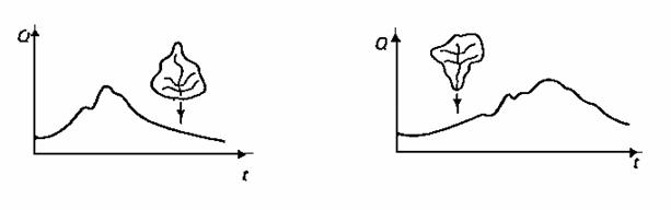
· Depends on soil structure of the drainage basin

Percolation is movement of water through the soil.

Precipitation moves water from the atmosphere to the ocean and land surfaces.

Runoff moves water from land surfaces to river channels for the return to the oceans. The water that flows over the surface into a stream has the greatest response to rain and snowmelt.

Amount of Runoff depends on:

Intensity and duration of a rain or snow melt event
Amount of water lost to interception and depression storage
Amount of water lost to infiltration
Characteristics of the drainage basin

When the soil particles and capillary water requirements are satisfied and soil particles are packed closely together, soil is saturated.

Transpiration moves water from the soil to the atmosphere via vegetation.

Loss of water in the cycle occurs from two sources:

Transpiration: plants draw water from the soil up through the roots and stem to the leaves and needles where water vapor is released to the atmosphere
Evaporation: water transfer to the atmosphere from soil, open water surfaces, and interception storage areas via a phase change from liquid to vapor

Snow melt is calculated from the simplified equation sm=MF(T-32) or snow melt rate equals a melt factor times the number of Fahrenheit degrees that the temperature departs from the freezing point. Melt factor is determined by examining past snow melt events in the region accounting for seasonal variations in solar radiation.

Streamflow consists of three components:

Baseflow
Interflow
Surface runoff

Water moves from the surface into the soil via infiltration, then percolates downward and is stored in the soil as soil moisture and groundwater.

Water Table is the upper surface of the ground water body.

Main Components of the Hydrologic Cycle

1. Rainfall - Water vapor in the atmosphere condenses into clouds and then falls to the ground as rain or snow

2. Runoff Generation - Rainfall reaching the ground infiltrates the ground, runs off to the stream channel, or evaporates into the atmosphere

3. Evapotranspiration - Rainfall on the ground and in the soil may evaporate depending on meteorological conditions. Water in lakes and streams may also evaporate back into the atmosphere. Plants transpire moisture back into the atmosphere through the photosynthetic process. The water used in evaporation and transpiration are lumped together into a single term, evapotranspiration

4. Streamflow - Water reaching the stream channel flows by gravity to the ocean

NWS hydrologic models use various techniques to simulate these components of the hydrologic cycle.

Hydrologic models used by the NWS to estimate runoff from an area are lumped parameter models. Lumped parameter models assume model parameters are homogenous over a basin or area. For input, these models use the average rainfall over the area, often called mean areal precipitation or MAP. Since rainfall is highly variable over an area and the NWS has few precipitation gages, the estimation of MAP is a difficult process.

Fixed Station Network

Most RFCs use a fixed data network of precipitation gages to estimate MAP. The RFC will use some method to determine the appropriate station weight to give to each station in or near a basin. Methods used to determine these weights include the:

Thiessen Method
Isohyetal Method
Grid Method

Thiessen Method

This section describes the Thiessen Polygon method or the grid-point weight method. Generally, the sum of the station weights for a basin will be 1.00. Gage sites in the basin will usually have higher weights than those outside the basin since they are generally more representative of rainfall in the basin.

Note: To compute MAP for a basin, multiply the daily rainfall for each station by its station weight and sum these values. The MAP can never exceed the highest rainfall measured.

Isohyetal Analysis

Another method of determining MAP is to draw isohyets, or lines of equal rainfall, for the storm. A planimeter measures the area within each isohyetal band. A weighted average precipitation can be determined for the storm period. This weighted average is the MAP. This method is time-consuming and not often used in real-time.

Using a Grid

Another method of computing MAP is to establish a grid system over a basin and have a rainfall report at each grid intersection. The arithmetic average of rainfall, either observed or estimated, for each grid point located in the basin would be the MAP.

Since there will not be a rainfall report at each grid point, an estimate must be computed. One method of estimating precipitation is the inverse distance squared (1/d-squared) method. In this method, divide the area of interest into four quadrants. The nearest station in each quadrant is an estimation of grid point precipitation. Each station has a weight proportional to the inverse of the square of the distance (d) from the observed data site to the grid point. The farther a site with observed data is from the grid point, the less weight that station has. The estimated precipitation can never exceed the maximum precipitation for stations used in the estimation.

NEXRAD

The National Weather Service Hydrologic Research Lab developed the Multisensor Precipitation Estimator (MPE) software to improve precipitation estimations used as input to the National Weather Service hydrologic models.

The program uses a combination of radar and gage based precipitation accumulations to produce gridded (4km by 4km) precipitation estimations. In areas beyond the range of NWS radars, only gage accumulations are used. When data is available, satellite based precipitation estimations are also included.

Forecasters at River Forecast Centers compare output from the MPE software with hourly rain gage reports to determine if bias adjustments are necessary to improve the precipitation estimations. RFC personnel must remove the false precipitation signatures radars often produce. In addition, forecasters look for erroneous rain gage reports and either corrects them or removes the reports.

Examples

Examples of areal averaging of precipitation by:

· Arithmetic Method

· Thiessen Method

· Isohyetal Method

ARITHMETIC MEAN:

1.46 + 1.92 + 2.69 + 4.5 0+ 2.98 + 5.00 = 3.09 in.

THEISSEN METHOD:

Observed precip (in)	Area* (mi²)	Percent total area	Weighted precip (in) (col 1 x col 3)
0.65	7	1	0.01
1.46	120	19	0.28
1.92	109	18	0.35
2.69	120	19	0.51
1.54	20	3	0.05
2.98	92	15	0.45
5.00	82	13	0.65
4.50	76	12	0.54
Totals	626	100	2.84

Average = 2.84 in.

*Area of corresponding polygon within basin boundary.

ISOHYETAL METHOD:

Isohyet (in)	Area* enclosed (mi²)	Net area (mi²)	Avg precip (in)	Precip volume (col 3 x col 4)
5	13	13	5.3	69
4	90	77	4.6	354
3	206	116	3.5	406
2	402	196	2.5	490
1	595	193	1.5	290
< 1	626	31	0.8	25
				0.1634

Average = 1634/626 = 2.61 in.

*Within basin boundary

Source: page 35, first edition, Hydrology for Engineers, Linsley, Kohler, and Paulhus

Exercises

Exercise 1

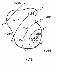
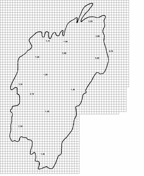
Using the Isohyetal Method, find the Average Precipitation.

The quality of the following graphic will depend upon the resolution of your monitor. The following precipitation values are on this figure, starting from the top: 2.20, 1.75, 2.00, 1.90, 1.60, 0.70, 0.80, 1.90, 3.50, 1.80, 1.40, 3.10, 1.40, 2.50, and 1.00. Count squares to obtain area.

Isohyet area – net avg volume
3.50	Answer	Units
3.00
2.00
1.50
1.00
<1.00
Average =

Answers should vary
Which is most accurate?

Exercise 2

Using the Thiessen Method, find the Average Precipitation. Compare your answer with the above Isohyetal Method.

Answer to the Exercise

Return to the Basic Hydrologic Concepts Menu of Lessons.

Updated 07/17/07