Probability is a number between 0 (never occur) and 1 (always occur) which represents how likely an event is to occur. Probability is normally defined in terms of the relative frequency of occurrence of an event from many, many trials.
Probability distributions or probability density functions (for example, Binomial, Normal, Lognormal, Gamma, etc.) describe the relative frequency of occurrence of data values when sampled from a population. There are continuous and discrete distributions (like random variables). Probability calculations for discrete distributions involve summation over the discrete variables. An example of a discrete distribution is:
| Binomial | used to describe the number of desirable outcomes (successes) in several repetitive and independent trials, when each trial results in either a success or a failure only. When the trial can have more than two outcomes, the multinomial distribution is used. |
Probability density functions (PDFs) for continuous random variables are:
| positive mathematical functions for all values of the random variable whose total integral is equal to 1, and where the |
| probability of the random variable to be less than or equal to a certain value a is equal to the integral of the PDF for values of the variable from negative infinity to a. |
| probability of the random variable to be between a and b equal to the integral of the PDF for values of the variable from a to b. |
| probability of the random variable to be greater than (to exceed) a certain value a equal to the integral of the PDF for values of the variable from a to positive infinity (Probability of exceedance). |
The PDF for a continuous random variables can be thought of as the histogram of relative frequencies plotted from an infinite number of observations with infinitesimally small intervals.
Examples of continuous probability distributions:
| Normal or Gaussian | Two parameter (mean and variance) symmetrical bell shape distribution. Probability of the variable to be within 1 standard deviation from its mean is 67%, within 2 standard deviation 95%, and within 3 standard deviations 99% |
| Log-normal | Two parameter (mean and variance in log units) symmetric distribution of log transformed values of a random variable |
| Gamma | Two parameter (shape and scale) asymmetric distribution |
Figure 1 shows examples of the fit of gamma and normal distributions to precipitation data whose distribution is asymmetric. Gamma distribution is a better fit to the precipitation histogram than the Normal distribution.
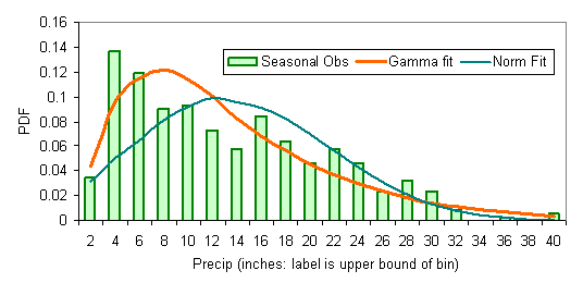 |
| Figure 1. Fit of Gamma and Normal Distributions to seasonal precipitation data at Olympia Airport, Washington. Mean = 12.5, standard deviation = 8.3, shape parameter = 1.97, scale parameter = 6.35 estimated from the seasonal data. |
REFERENCE:
Wilks, D.S., 1995. Statistical Methods in the Atmospheric Sciences. Academic Press. Pages 64 -93