
Radar Reflectivity Measurement
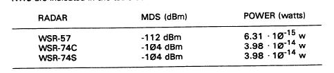
As for the WSR-88D, the useable MDS nas been calculated the be in the area of -112 dBm (6.3 1015 w). This is a preliminary figure, and is subject to change, based upon the characteristics of the production radar systems. [OSF - 1989 - J. Hunt] Even so, each system is an "individual" and as a result, the useable MDS will vary somewhat from one WSR-88D to another.
- Detection Of Precipitation
The degree of detection of precipitation targets is dependent on a variety of factors. Important among these are: Atmospheric conditions between the radar and the target, distance from the radar to the target, target characteristics, and radar characteristics.
Conditions in the atmoshpere and the actual character of a given target are unknown quantities. The power being returned to the radar from a target has been previously referred to as reflectivity. It is a measure of the efficiency of a target in intercepting and returning radio frequency energy. Thus, a weather radar system provides a value of "efficiency" with which targets in the atmosphere return the energy transmitted by the radar. And this efficiency is measured in terms of reflectivity. The big unknown for the radar meteorologist concerns the precise characteristics of the precipitation target itself. For example, what is the size and size-distribution of the precipitation particles in the target?. How would the size effect the backscatter? How much of the precipitation is in liquid state, and how much is in a frozen state? How would this effect the power returned?
Unless an observer in an aircraft (conducting detailed studies of
the target) could immediately communicate the answers to these questions
(and others) to the radar operator, he must simply compare the strength
of one return with another. When this comparison is completed, an estimate
of the relative
effects of the echo may be made. The radar operator must be aware of certain assumptions which must be made with regard to particle size, distribution, state (ice, liquid, or mixed) of the target, etc. Because the atmosphere is a dynamic target, comprising innumerable possibilities of characteristic variations, radar ref lectivitv values received must be based on several assumptions. In this module, we will examine some of these, and apply them to the values of reflectivity upon which the radar operator must rely.
The radar characteristics and the distance to the target are known
quantities, and their effect on the signal strength returned from a given
precipitation target may be calculated. Here in this module, we will examine
these known (and calculable) effects. Thereupon, we'll apply them (along
with the assumptions mentioned above) to a standard formula
which is used to determine the reflectivity for a given radar system.
- The Radar Equation
The conventional weather radar systems used in the National Weather Service (WSR-57, WSR-74, etc.) actually measure only two (2) basic quantities. These basic measurements are...
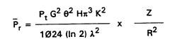
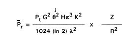
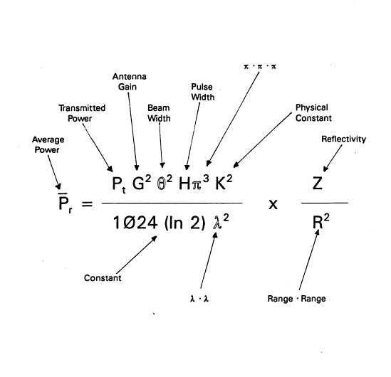
The following paragraphs describe the variables of the Probert-Jones equation which are known or calculable. Refer to the Foldout drawing (Page 11-1 lA)...
Pr is the average echo return power. Note that the Probert-Jones equation interprets average returned power. This is a power value which is calculated from information received from more than one pulse of energy. Conventional NWS radar systems use either 15 or 31 successive pulses of RF energy to determine an average power return from a given location in the atmosphere. Averaging is necessary since the power returned from a meteorological target varies greatly from pulse to pulse. A sampling scheme (rate) may vary from radar to radar.
is the power transmitted from the radar in the outgoing energy burst. The average return power varies directly with the Pt. As a result, a doubling of the transmitted power (with no other changes) would double the average returned power. Cutting Pt in half would result in half the average return power.
G is the gain of the radar antenna. Antenna gain is a measure of the ability of an antenna to focus energy into a beam for both the transmitted and received electromagnetic waves. As discussed in earlier sections of this package, the WSR-57 antenna has a Gain of 38.1 dB (a factor of 6,460). The WSR-88D antenna has a gain of 45.5 dB (a factor of 35,480). The power received from a given target varies directly with the SQUARE of the antenna gain. This means that doubling the antenna gain would result in four times the original energy value. On the other hand, if the gain were to be halved, the return power would be cut to 1/4 of its original value.
6 is the antenna beamwidth. According to the Probert-Jones equation, return power increases directly with the square of the beamwidth, just as for antenna gain. There are other considerations which will come into play in this regard, and we will discuss them later.
H represents the pulse width of the transmitted RF energy. The received power will vary directly with the pulse width. The WSR-57 utilized two (2) different pulse widths (0.5 uS and 4.0 uS), and the WSR-74C uses a single pulse width. The WSR-88D is capable of pulse widths of 1.57 uS and 4.5 uS.
R is the range to the target. The reflected energy reaching the antenna varies inversely with the square of the distance to the target. As an example, a target at 100 miles would return only ¼ the energy as it would if it was at a distance of 50 miles. This occurs because the power density of an electromagnetic
wave is proportional to 1 — R2 (the reciprocal of the square of the range). This drop-off of returned power is also referred to as range attenuation. Recall that in the WSR-57 and WSR-74 radar systems, we compensate for this law of physics by "normalizing" the received data in the STC circuits of the digital video integrator processor (DVIP). The method used adds 21 dB to VIP level 2 signals (and greater) which are less than 20 km or greater than 230 km in range. Signals between 20 km and 230 km in range are modified in a way that compensates for the range attenuation function. A specific value is added to the received data value as a function of the range between 20 and 230 km.
![]() is the wavelength
of the RF energy expressed in meters. The amount of power received varies
inversely with the square of the wavelength. To state this in terms of
current NWS radars, a "C" band (WSR-74C) radar will have ¼ as much
returned power than an "5" band radar (WSR-57 or WSR-88D) if all other
parameters are the same. They, of course, are not. Short wavelengths
(under 10 centimeters) are subject to significant attenuation (loss of
signal intensity) in the atmosphere, and are not suitable for use in a
wide-area surveillance network. This is why the '74C radars are relegated
to a "local warning" role in the NWS.
is the wavelength
of the RF energy expressed in meters. The amount of power received varies
inversely with the square of the wavelength. To state this in terms of
current NWS radars, a "C" band (WSR-74C) radar will have ¼ as much
returned power than an "5" band radar (WSR-57 or WSR-88D) if all other
parameters are the same. They, of course, are not. Short wavelengths
(under 10 centimeters) are subject to significant attenuation (loss of
signal intensity) in the atmosphere, and are not suitable for use in a
wide-area surveillance network. This is why the '74C radars are relegated
to a "local warning" role in the NWS.
1024 (In 2) and are mathematical constants. 1024 (In 2) is sometimes
expressed as 210 (In 2), where "In" means natural logarithm. 1024 the
natural logarithm of 2 is 709.7827129. (Pi) of course, has a value of
3.141 592654 ish. has a value of 31.00627668 ish.
K is the final "known" factor in the equation. It is described as
the physical constant, and is used to represent the "type" of target from
which the radar is receiving backscattered energy. The value describes
the physical properties of the reflecting substance; especially the ability
of the substance to transmit electrical current (electrical "conductivity").
The power received is proportional to K2. For example, if the target "substance"
is liquid water, then K2 ranges from 0.91 to 0.93 as the ![]() varies from 1 cm to 10 cm. If the target is ice, a K2 value
of 0.18 is used. For these (ice) targets, the
varies from 1 cm to 10 cm. If the target is ice, a K2 value
of 0.18 is used. For these (ice) targets, the ![]() of the radar is not a significant factor. NWS radar systems use a K2
value
which describes liquid water targets. Because of this, power received from
reflecting particles composed entirely of ice (except for those which are
extremely large) will be about one-fifth (20%) of the power value received
from liquid targets. This situation results in rather large underestimates
of the water content of snow and ice crystals, when these particles are
detected in the radar beam. Additionally, these "solid" targets may not
even be detected at long radar ranges.
of the radar is not a significant factor. NWS radar systems use a K2
value
which describes liquid water targets. Because of this, power received from
reflecting particles composed entirely of ice (except for those which are
extremely large) will be about one-fifth (20%) of the power value received
from liquid targets. This situation results in rather large underestimates
of the water content of snow and ice crystals, when these particles are
detected in the radar beam. Additionally, these "solid" targets may not
even be detected at long radar ranges.
The Reflectivity Factor is represented in the equation
as Z. If all of the assumptions of the radar equation (to be discussed
shortly) are met, then there are two (2) important characteristics of a
LIQUID precipitation target which determine how efficiently it returns
power to the radar. These are...
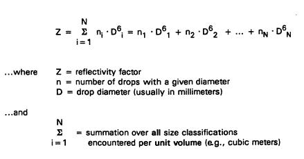
The reflectivity factor of a Precipitation target is determined
by the SUM of the
SIXTH POWER of ALL drop diameters (usually measured in millimeters)
in the
SAMPLED VOLUME.
Target reflectivity increases rapidly as the drop size grows, even
though the total water content may remain essentially the same.

In order to evaluate the received energy collected by a radar, considerations
must be given to some of the limitations encountered in radar observations.
Some of these limitations result from a number of assumptions which are
applied to the radar equation. For example, it is assumed that
An additional limiting factor of weather radar requires consideration
at this point in our discussion of reflectivity. Recall that the beamwidth
(8) used in meteorological radar systems is relatively narrow in both the
vertical and horizontal axes (1.60 for the WSR-74C, 2.00 for the WSR-57,
and 0.950 for the WSR-88D). In the drawing below (WSR-74C radar beam at
an elevation angle of 1 0), notice that the beam spreads to a diameter
of about 6,950 feet at 50 nautical miles. and to around 17,300 feet at
100 nautical miles.
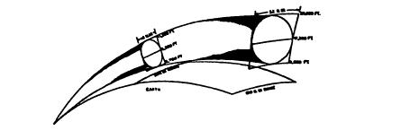
At 50 nmi, the beam extends from 2,700 feet in altitude to about
11,200 feet. At 100 nmi, the lower edge of the beam is 8,800 feet above
the earth, and the top edge is at an altitude of about 25,800 feet.
Values of radar reflectivity in the Probert-Jones equation are (in
part) based on the assumption that precipitation is filling the
entire beam. Because of this rather narrow beam characteristic of weather
radar, and due to the relatively broad area of most precipitation targets,
"beam-filling" certainly does not occur.
The figure below shows that a precipitation target near the radar
site (target "A") is "filling" the radar beam, while a similar target ("B")
at a greater distance does not fill the beam. It is obvious that target
"B" will reflect a smaller amount of energy back to the radar antenna.

Because many precipitation targets generate echo "tops" below 20,000
feet, it is apparent that the radar beam may not be filled with precipitation
at greater distances, Additionally, high-based thunderstorms present beam-filling
difficulties, especially at close ranges. In both cases, underestimates
of precipitation may well be the result.
In widespread stratiform precipitation, beam filling needs to be considered only in the vertical axis. For the detection of showers and thunderstorms, both the horizontal and vertical effects of beam filling must be appraised. Some showers are less than a mile in width, and even a 1 0 beam at 60 nmi may not be completely filled. In addition, the most intense portion of a storm (a core) may cover only a small area within the storm.
The Probert-Jones radar equation is shown again below. Notice that
there is no variation provided for in the variable 02. It is simply a parameter
for a given radar system, and is taken with the assumption that the total
energy in the beam is playing a part in the backscattering of target echoes.
Notice also that all of the parameters of the equation which describe
any radar system share the same "fixed" value. "K2" is the only
real variable.
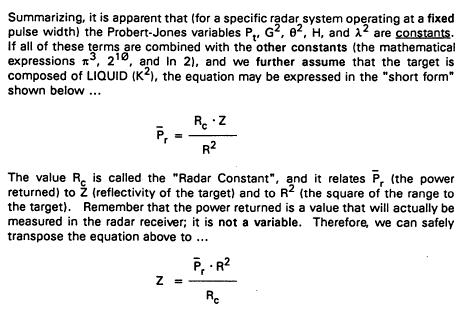
This even more simplified equation simply states that the reflectivity
is equal to the power returned times the square of the range divided by
the radar constant. To state the radar precipitation measuring function
in specific (yet still simple) terminology, a given radar
Such estimates of precipitation target reflectivity are accurate
only if the assumptions of the radar equation are met. Again, seldom is
this the case. A reflectivity value which is derived in this way is referred
to as
and is a value that is unique to each individual weather radar
system.
![]()
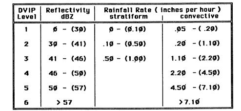
Precipitation targets produce a range of dBZ values from 0 in very light rain to in excess of 60 in extremely heavy rain and/or hail. Without knowing the precise nature of the targets at the far end of the radar beam, the radar system uses the measured average returned power to estimate the equivalent reflectivity (Ze) of all targets. Traditionally, Ze values have been grouped together in six (6) distinct ranges. These are shown in the table below. The six ranges of reflectivity correspond to the digital processor (DVIP) threshold levels which are used in the WSR-74 and WSR-57 radar systems.
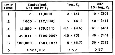
The DVIP levels of equivalent reflectivity are shown in mm6 (millimeters raised to the 6th power) and in dBZ. The values in parentheses indicate thresholds for the next higher level (45.7 dBZ would be a Level 3; 46.0 dBZ would be a Level
4). The decibel representations are much easier to use than are the
Ze values.
The logarithmic (base 10) functional notations of reflectivity values are very convenient for use because the physical power relationships of electronic signals found in a radar system's receiver follow the very same relationship.
In WSR-74 and WSR-57 systems, the reflected power is amplified in
logarithmic receiver circuitry, and processed in digital equipment (DVIP
systems) which integrate the average power returns from each desired atmospheric
volume. Thus, the reflectivity (Ze) values may be represented in "ranges"
of values specified by the DVIP levels in the table on page 12.
The radar display system is driven by video voltages which represent each
of the six DVIP levels. This allows the radar operator to easily "quantize"
the reflectivity of the meteorological targets being displayed on the radar
scope(s).
- Reflectivity / Rainfall Relationships
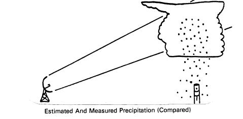
The relationship between equivalent radar reflectivity (Ze) and rainfall
rate has been widely investigated over the years, and there are many refinements
which are yet to be made. With established NWS radar systems, estimates
of rainfall frequently require subjective modification by the operator
in order that they fall within a range of reasonable accuracy. The basic
relationships between reflectivity and rainfall are based upon empirical
studies, where rainfall rate is measured at the earth's surface while equivalent
reflectivity is simultaneously being estimated by the radar looking at
precipitation targets located directly above the rain gage. Refer to the
figure below
Numerous variations of the relationship between reflectivity and
rainfall (Z-R) rates have been developed from past studies of the subject.
Many of these studies have centered on liquid (as opposed to ice or ice-covered)
precipitation. If the particle size distribution were a unique function
of the precipitation rate, a universal Z-R relationship would exist. However,
these studies have abundantly demonstrated that there is no such unique
particle size distribution for any given rainfall rate. Based upon many
studies, the NWS has adopted the following two Z-R relationship values
· Ze = 200R1.6 (for stratiform precipitation)
· Ze = 55R1.6 (for convective precipitation) where
Ze is equivalent reflectivity in mm6/cm3
· R is the rainfall rate in millimeters per hour.
Equations like those shown above are called reflectivity/rainfall equations, or simply "Z-R Equations". They are defined as follows
· Ze = 500R1.5 (thundershowers)
When rainfall rates are converted to inches per hour, the
Z-R relationships used by NWS yield the values shown in the table below
The table depicts rainfall rates as a function of both Z-R relationships
/used by the NWS. Notice that convective targets generally tend to produce
higher precipitation rates than do stratiform targets at the same DVIP
level.
When the sampling volume contains hail, the Z-R equations used for the standard NWS table above do not accurately represent the precipitation rate. The variability of the size of hailstones as well as the extent and thickness of water coating (if any) have a large effect on the returned power. In addition to being highly variable, reflections from hail targets are usually much stronger than those from liquid precipitation. The result is that rainfall rates will be underestimated unless the radar operator can determine (by other means) that hail is present in the storm. Other factors which can cause underestimates of rainfall are distant targets, small targets, wide radar beams, subrefraction of the beam, attenuation by intervening targets, and wet radomes. The first three of these are a direct result of a target not filling the radar beam. Subrefraction is an effect in which the radar beam may be "bent", causing the energy to propagate over a target. The attenuation factors will depend upon the extent (and intensity) of precipitation between the radar and the desired target. Radome wetness attenuation is usually small, but may become significant if the exterior of the dome is not well maintained (clean, painted, etc.).
All of these possible factors must be considered by the radar operator,
based on a knowledge of the radar equipment and the ongoing weather situation.
- WSR-88D Reflectivity Measurement
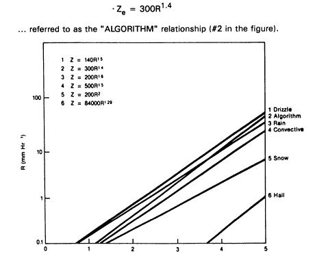
Considering the previous Z-R discussion (many possible reflectivity-rainfall rate relationships), the WSR-88D software has been designed to utilize a set of multiple Z-R equations. The figure below depicts various Z-R relationships, one of which has been selected as the WSR-88D default equation
Log10Z
The rationale for the "Algorithm" Z-R equation is that it should provide a good average for different precipitation types. The design of the WSR-88D system was conceived with the idea that a mean bias adiustment will be applied by the hydrologic software to rainfall estimates, based upon data collected from an "umbrella" of precipitation gages. The gages will report data to a central computer system, which will relay the measured precipitation to the WSR-88D.
This method of verification of rainfall (and subsequent real-time modification of the WSR-88D algorithms) requires a substantial number of gaging stations located within the radar's range. There is some question as to whether an ample number of gages will ever be installed. The WSR-88D default Z-R equation (Ze = 300R1.4) will be utilized in any case, and will probably be subject to change during the life span of the WSR-88D radar system.
The WSR-88D hydrologic software contains sequential sub-functions which are used to compute derived products of 1-hour, 3-hour, and storm total precipitation accumulation. The five processing functions are